Python Scripting

Background

Python is the programming language used by ArcGIS that allows for additional operations and tools to be used. An experienced Python user can perform advanced techniques of analysis that would not be possible without this training. Because of this, it is extremely useful to have at least some experience using Python.

Goal

Our objective was to get an introduction to using Python by writing several basic scripts for simple functions in ArcGIS. These are the three scripts that we did finish during the course of the semester.

For each script, I include a screenshot from PyWin and also text so that the script can be copied.

Figure 1 - Clip script

The first script was a simple clip tool (figure 1).

import arcpy
arcpy.env.workspace = W:/geog/CHupy/geog337_f13/HAASTA/Exercise02
arcpy.Clip_analysis("lakes.shp", "basin.shp", "Results/lakes_myClip.shp")

Figure 2 - List of features

The second script (figure 2) was to display a list of all the features in a feature class, as well as the type of feature
(point, line, polygon).

import arcpy
from arcpy import env
env.workspace = "W:\geog\CHupy\geog337_f13\HAASTA\Exercise_Data\Exercise07"
fclist = arcpy.ListFeatureClasses ()
for fc in fclist:
    fcdescribe = arcpy.Describe (fc)
    print fcdescribe.name + " is a " + fcdescribe.shapeType + " feature class "

Figure 3 - Airport buffers

The last script involved creating a series of buffers around different types of airports (figure 3).









import arcpy
from arcpy import env
env.workspace = "W:\geog\CHupy\geog337_f13\HAASTA\Exercise_Data\Exercise07"
fc = "Results/airports.shp"
airport = "Challenge/airport_selection.shp"
seaplane = "Challenge/seaplane_selection.shp"
where_clause = '"FEATURE" = \'Airport\''
arcpy.Select_analysis (fc, airport, where_clause)
where_clause = '"FEATURE" = \'Seaplane Base\''
arcpy.Select_analysis (fc, seaplane, where_clause)
airportBuffer = "Challenge/airport_buffer.shp"
seaplaneBuffer = "Challenge/seaplane_buffer.shp"
arcpy.Buffer_analysis (airport, airportBuffer, "15000 METERS")
arcpy.Buffer_analysis (seaplane, seaplaneBuffer, "7500 METERS")

Conclusion

Python is a very helpful, though tough to learn, tool. Having no background at all in programming languages, I struggled somewhat when doing these exercises. Also, it was at the beginning of the semester that I wrote these, so I apologize for not being able to elaborate more on each individual script. I simply didn't document the process well enough at the time. However, I did find that I enjoyed working with Python and I realized that it can be an incredibly helpful tool in the right hands. I would very much like to continue my education in this area, as it will compliment the other GIS skills I have learned this semester very well.

Frac Sand Mine Suitability and Raster Modeling

Goals and Objectives

This exercise was the culmination of the frac sand mining exercises we have been doing all semester, as well as an exercise in raster modeling. Using data we gathered in previous labs, we were to make a suitability model for frac sand mining in Trempeleau County by overlaying various raster data. We also found where high risk areas for mining were in the county.

 

Part 1

Methods



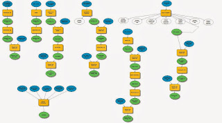
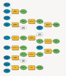
Figure 1 - Work flow for part 1

It was necessary to use many different tools and data sets to compile the information needed to find suitable mining areas. The exercise was broken up into two parts: suitability and risk. For part one, we had to find suitable areas for mining using hill slope, geology, water table depth, land cover types, and proximity to railroad depots. We found these suitable areas separately, then used the tool 'raster calculator' to combine them into one suitability map. Figure 1 shows the work flow for this portion of the lab.






Figure 2 - Suitable geology for frac sand mining

For each map, we ranked suitability from 1-3, 3 being highest and 1 being lowest (or 0 being unusable) by reclassifying the raster data. For consistency, I used green for rank 3, yellow for rank 2, and red for rank 1 on all the maps.

 When deciding what areas are suitable and what areas are not, it can vary from person to person. Geology, however, does not. Wonewoc and Jordan sandstone formations are suitable, so I did only one rank for that map (figure 2).








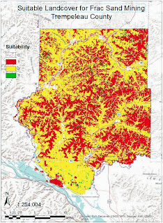
Figure 3 - Suitable land cover sites

For land cover, I ranked the suitable types by what areas were easiest to clear before mining can begin. This means that rank 3 included barren, shrub, and grass lands, Rank 2 was pasture and crop lands, and rank 1 was any type of forest land. I excluded any developed areas and wetlands entirely. Figure 3 shows the result.


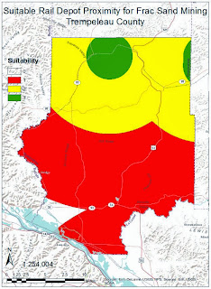
Figure 4 - Suitable distance from rail depots

Any sand mine will need a way of transporting the product, so we made a map showing suitable distance from rail depots. Rank 3 locations were any areas within 3 miles of a depot, rank 2 was between 3 and 10 miles away, and anything farther was rank 1. The map units were in meters, so I used the meter equivalent of these mile distances. To do this, I ran the 'euclidean distance' tool. Most of the maps I made only involved data that fell within our study area. However, I would think that frac mines in Trempeleau County would still be able to utilize rail depots in neighboring counties, so I included them when I ran the tool. It was only after I got the result that I used 'extract by mask' tool to show only suitable areas within our study area. I did have a mask set in the Environments menu, but it seemed to only work selectively, so I still had to run the tool occasionally. Figure 4 shows the result.





 

Figure 5 - Suitable slopes

 Hill slope is important when deciding an area to mine. Rank 3, the areas in green, are the most suitable areas with the lowest slope. The steepest areas in the study area are in red. Using a mosaiced DEM from a previous lab, I ran the slope tool and reclassified it to get the result in figure 5.

Once the sand has been mined, it must be washed to remove unwanted particles. For this reason, building a mine where the water table is close to the surface is preferable. Figure 6 shows where the water table is closest to the surface in green.


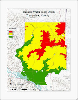
Figure 6 - Suitable water table depth



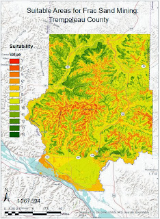
Figure 7 - Part 1 suitable areas











Results

Once I had the five separate suitability maps created, it was time to combine them to make one overall suitability map. To do this, I used the tool 'raster calculator' to add the values of all the layers. Since we used a constant suitability scale (0-3), the raster could be added together to give a range of suitability. Figure 7 shows the most suitable areas for frac sand mining in Trempeleau County, factoring in hill slope, water table depth, geology, distance from rail depots, and land cover type. As you can see in figure 7, the Northwest portion of the study area contains the most suitable areas for mining.

Part 2

Methods

Figure 8 - Work flow for part 2

Part two involved finding areas where mining would have the most impact, thus the most risk. This included proximity to streams, prime farmland, proximity to residential areas, and proximity to schools. I realized after creating the final risk map that I classified them backwards. The exercise called for ranking areas with highest risk at 3, and lowest risk at 1. I did all the maps in this section with low risk areas at rank 3 (thinking that low risk would be a more suitable area). Even with this mistake, risk can be clearly seen in the following maps. Figure 8 shows the work flow from Model Builder that I used.













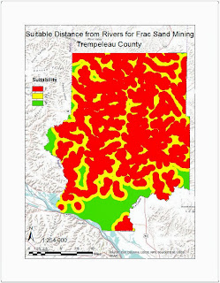
Figure 9 - Suitable distance from major rivers

There are many streams in the study area, and including all of them in this analysis would mean that there is no suitable area. I chose only primary perennial streams, since risk to these streams would have a larger effect on the area. I again used the 'euclidean distance' tool to create a raster ranking distance from streams, then reclassified it to have only three classes. Figure 9 is the finished map. As you can see, Trempaleau County has a great deal of rivers, making it difficult to find suitable areas.













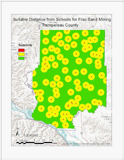
Figure 10 -  Risk index for area schools

Because some people may not want a sand mine near schools for various reason, Figure 10 shows the risk model for schools within the study area. Rightfully so, schools are spread out evenly across the county, so in this case there is no specific region that stands out as more or less suitable. There is more than enough space between schools (shown in green), however, for mining. We also wanted to keep risk to prime farmland to a minimum. Figure 11 shows this risk map.


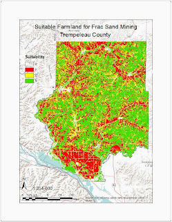
Figure 11 - Risk to prime farmland from frac sand mining.

 




Results

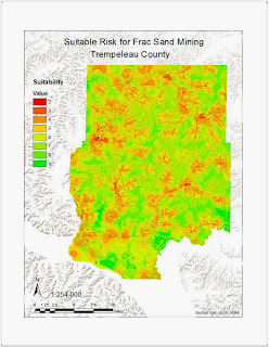
Figure 12 - High-low risk areas for mining. Red
represents areas of high risk, green is low risk.

Figure 12 is the final product from part two. Again, the ranking is backwards from what we were supposed to use, but the map still does show areas where sand mining would put local areas at risk. This map was made by once again using the 'raster calculator' tool to combine the risk maps I had created by adding the pixel values.





 We were also tasked with using the 'viewshed' tool to find if suitable mining locations would be visible from areas of our choice. I used the campground feature class to run the tool on. In figure 13, purple denotes what is visible from these campgrounds. This is overlaid on the final suitability map made by combining the products of parts one and two. Figure 14 is the finished product.



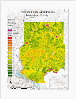
Figure 13 - Viewshed of Trempeleau County campgrounds






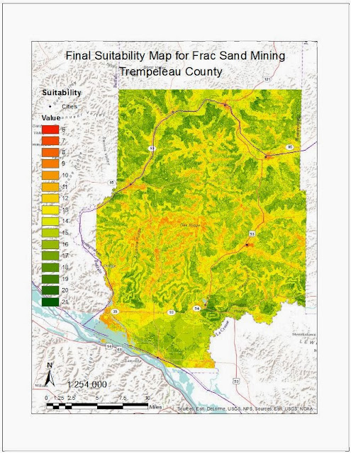
Figure 14 - This map is the final suitability map for
Trempeleau County including parts 1 and 2

Conclusion

 

I learned a great deal not only about using and interpreting GIS data, but also about frac sand mining during the course of this lab. Frac sand mining is a huge (and controversial) industry in Wisconsin. This was a lengthy exercise, but it tied everything we did this semester together very well. From my studies this semester, it seems that the northwestern portion of our study area would be the best place to scout new areas for frac sand mines.





 

 

 





Network Analysis

Goals and Objectives

The goal of this lab was to learn and practice network analysis skills while continuing our research of frac sand mining in Western Wisconsin. For this exercise, we were tasked with finding the shortest route from each mine/processing plant to the closest railroad terminal. We then had to calculate the cost of road maintenance due to frac sand trucks using these routes, broken down by county.

Data

Street Network Dataset - ESRI street map USA
Western Wisconsin frac sand mines - Point feature class geocoded by our class during previous lab
Railroad Terminals - Point feature class provided by instructor

Methods

Some of our geocoded mines are also a rail loading location. The first step was to exclude these sites from our analysis, as they would not require and road travel to bring their product to a rail terminal. Once I did this, I created separate shapefiles for mines that would require road travel and for mines that have rail loading locations. Then I merged the mines with rail loading with the rail terminals shapefile (mines could transport their product to a mine with rail loading, even if owned by different companies) so that I had one shapefile containing all locations where product can be loaded onto a train.

Next I created a network analysis. I used the closest facility function to find the closest rail terminal to each mine. The points in the mines shapefile were set as the incidents and the points in the terminal shapefile were set as the facilities. Flipping those around would create a network analysis that creates routes from the terminals to the closest mine, which would be unhelpful for our purposes.

Figure 1 - Model Builder work flow

Using model builder, I exported my route data as a shapefile and found a way to calculate total miles driven on roads, as well as the cost the county incurs each year for road maintenance (Figure 1). The first part of the model (up to the "Solve Succeeded" bubble) is for creating and exporting the closest route data. All steps after that were to calculate miles driven on road and cost incurred to each county. To do this, I intersected the route data with my selected counties. This not only figured in only the mines and terminals in Western Wisconsin, but also merged the tables so that I had a county field with my route data. This was needed so that I could calculate distance and cost for each county separately. Next, I summarized the Shape Length field by county.

Equations:
Yearly Cost Per County = [Sum_Shape Length] (This is the total length of all routes in the county in meters) * .0006271 (This converts distance from meters to miles) * .022 ($.022 is the maintenance cost per mile) * 100 (This is the amount of trips every year on each road: 50 trips, both ways)
(The maintenance cost per mile and the amount of trips made every year are hypothetical figures)

Results


Figure 2 - Map of mines, rail terminals, and the truck routes to the nearest terminal



Figure 3 - Table showing results from calculations

Figure 4 - Miles driven every year by trucks transporting frac
sand to rail terminals, by county

I created a map showing the results of the network analysis (Figure 2) as well as graphs showing the results of distance and cost calculations for each county (Figures 4 and 5 respectively). Figure 3 is the table used to create figures 4 and 5. As you can see, Jackson county will have to spend the most money on road upkeep at $744 per year, followed by Trempealeau county at $650 per year.



Figure 5 - Cost of road maintenance incurred each year by
transporting frac sand to rail terminals, by county

Trempealeau county has a very large number of frac sand mines, meaning more trucks on the road. Jackson has fewer mines than other counties, but longer distances to travel to get to the nearest rail terminal. the mines located in the southeastern part of the county are routed to the opposite corner of the county. The highway used even runs parallel to a rail line for a portion of the trip, and so the damage to roads could be greatly reduced by constructing another rail terminal in this section of the county.

Conclusion

Before this exercise, I had never used Model Builder or Network Analysis. Both are extremely useful tools that I hope to utilize even more in the future. The actual results are hypothetical, as the cost and mileage data were hypothetical. Also, I assume that in the real world specific routes are altered and updated as necessary. But I think this is an accurate look and the counties relative to each other. Jackson and Trempealeau counties probably do have higher road construction costs due to the high number of frac sand trucks that use those roads everyday. The skills I learned in this lab are therefore very useful in Wisconsin.

Data Downloading and Geodatabase Design

Disclaimer

The following post is out of order. Creating a geodatabase and acquiring data would be the first logical step. Due to a federal government shutdown shortly after our class began this exercise, we were forced to put this important step on hold as most of our data was to be accessed from federal government websites. Please keep in mind that, under normal circumstances, this post would precede my geocoding post.

Goals

The goal of this exercise was to become familiar with acquiring geospatial data from various sources on the Internet, then importing this data into ArcGIS for use and interpretation. During this process, we were required to design and set up a geodatabase for storing all this data, as well as make sure everything was projected in the same coordinate system.

Methods

The first data set I downloaded was the railroad data from the National Atlas website. This data, like the others, was compressed in a zip file and had to be unzipped before use. Next, I visited the National Map Viewer website at http://nationalmap.gov/viewers.html. Here, using the interactive web map, I selected Trempealeau County. There were several data sets available, but I downloaded only landcover and DEM (Digital Elevation Model) data. From the USDA Geospatial Data Gateway (http://datagateway.nrcs.usda.gov/), I downloaded cropland data for Wisconsin. Lastly, I downloaded soil survey data from the USDA soil survey website (http://websoilsurvey.sc.egov.usda.gov/App/HomePage.htm).

Other than just unzipping it, some of the data had to be manipulated somewhat before it could be used. The elevation data was sent in two separate raster files so that a singe image wasn't too large of a file. In order to make one DEM raster image, I ran the mosaic to new raster tool. This created a single, uniform image that covered Trempealeau County.

I decided to use NAD 1983 Wisconsin Transverse Mercator for my projection, as this one would work best to display the whole state of Wisconsin. After I had that decided, I created a geodatabase and imported all of the data I had acquired. I also created a feature data set for the natural resource feature classes.

Results




Figure 1 - Data obtained from government websites

Figure 1 shows a very basic image of the different data we downloaded with the railroad layer on all of them. I used the spatial analyst tool to show only data within Trepeleau County, however this tool did not work on the map of crop land. The tool negatively affected the colormap of the image, and the data was not portrayed as well. I left it as is for now.





Geocoding

Goals and Objectives

The goal of this exercise was to learn the process of obtaining data in the form of a spreadsheet and geocoding that data in ArcMap. We were to download an excel file that contained the locations of frac sand mines in Wisconsin from wisconsinwatch.org and display the addresses on our map.

The data was not able to be geocoded right away. The addresses were in different forms; some were street addresses, some PLSS locations, and some just had directions like "west of Augusta." Our objective was to map these locations as accuratly as we could.

Methods


Figure 1- Data table prior to being normalized.

Because of the inconsistancy of the data, I first needed to normalize the table so that each location had a street address, city, county, and state in seperate fields. Figure 1 shows how the data appeared before I worked on normalizing it. When running the geocoding tool using this table, almost no locations were matched. The ones that did match were mostly wrong.

Figure 2 shows a sample of my data after normalization. By using a combination of aerial photo interpretation, websites referencing specific mines, Google Earth, and mapquest.com, I was able to come up with a street address for each location.

Figure 2 - Normalized addresses.

When I ran the geocoding tool using this new normalized table, I had much greater success. All 14 of my mines were "matched," however some of them were in the wrong locations. For those, I simply used the "pick address from map" option and moved the point.



Figure 3 - Map showing my geocoded mines and those done by classmates

Results


Each mine had its own "unique ID" so that we could keep track of them. Classmates of mine had geocoded some of the same mines that I had. By merging all of the classes geocoded mine shapefiles together, then running a query and selecting those mines that had the same unique IDs that I had used, I created a layer that was made up of mines that should have been the same addresses as the ones I had geocoded. Just by glancing at figure 3, it's easy to see that simple errors can cause drastically different outcomes.

Figure 4 - Distance (in meters) between points.

Figure 4 is a table that shows the distance between my mines and the closest mine to it. The problem with this is that there is no way to get the tool to calculate the distance between my mine and the ones that have the same unique ID. We have to assume that the distance shown in the table to the closest mine is the same mine. Usually, this is probably the case. In some situations, however, a mine could have been geocoded to as far away as a different county.

Discussion

Some of these errors could be inherent, such as issues when changing the projection of a shapefile, but most of the discrepancies are operational errors. Operational errors occur when managing and processing the data. Inputting the wrong address, misinterpreting data, or selecting the wrong location from aerial photography are all situations that could lead to the sizable distance between some of these mines (Lo and Yeung, 2006). The only way in which we can know for sure what points are correct would be to contact the owner or manager of the mine, or visit the facility personally.

Conclusion

During this lab, I have learned the different ways to geocode, as well as the importance of normalization. I also realized how big of a difference seemingly small mistakes can make. Calculating point-distance is an interesting tool that will come in useful in the future, which I did not even know existed before doing this lab.

References

Lo, C.P., Yeung, A.K.W., (2003), Concepts and Techniques in Geographic Information Systems. (pp. 107-108). Pearson Prentice Hall.

Brief Introduction to Frac Sand Mining in Wisconsin

Intorduction

Locations of major shale gas resources

Wisconsin has an abundance of sand deposits, mostly concentrated in the west-central part of the state. This sand has been mined for hundreds of years for production of various products including glassware, mortar, and cement. Sand mining in Wisconsin has dramatically increased in recent years for use in hydraulic fracturing (fracing), a technique used for obtaining oil and natural gas from the earth. The frac sand is mined and processed in state, and shipped out to areas of the country where drilling operations are taking place. Texas, Oklahoma, and North Dakota are just a few of the places utilizing this technique.

Over the course of the semester, our GIS II class will be focusing our projects on studying the various facets of this booming industry, which I will be documenting in this blog. Our studies will be concentrated on Trempealeau county, as this area features some of the most frac sand operations.

Hydraulic Fracturing

Diagram of hydraulic fracturing operation

Fracing is the process of drilling a standard oil well, and using explosives to crack the bedrock. After the rock is cracked, water, chemicals, and sand are pumped into the well under high pressure to pry open the cracks, and the sand is left in the wound to hold it open. This creates a permeable area to extract oil or gas. 

Though fracing is in Wisconsin news more and more these days, it is not a new technique. Fracing has been used since the mid 20th century. The reason for the recent surge in demand for frac sand is that new horizontal drilling technology has been introduced, allowing for access to many deposits of resources that have long been out of our reach. This technology, combined with our ever-growing need for fuels, has made frac sand a huge industry in Wisconsin in just a few short years.

Sandstone locations and frac sand facilities in Wisconsin

Frac Sand

Fracing uses a very specific type of silica sand, popularly known as quartz. Sand used for fracing operations must be almost entirely quartz, rounded, and of a very specific size. Wisconsin has some of the best frac sand deposits in the country, which is why the excavation of this sand is such a huge (and controversial) topic in the state. Sandstone deposits suitable for frac sand are mostly concentrated in the western part of the state. As you can see in this map, Trempealeau county contains a large number of these mines and processing facilities, which is why we are focusing our studies here.

Impacts of Frac Sand Mining in Wisconsin

As was mentioned earlier, frac sand mining is a controversial topic. As with any industry, there can be impacts (good and bad) on the people, wildlife, and environment of the area. These impacts can vary from one mine to another depending on size of the operation, surrounding geography, and local population. 

Air pollution is always a large concern. As with any industrial setting, there will be some emissions. All the heavy equipment used to excavate, process, and eventually transport the product means a large increase in gasoline use and the emissions that come with it. There is also the issue of dust. With the amount of heavy equipment moving around, blasting of rock, and bare sandstone exposed, dust can get into the air. On a windy day, this dust may travel far away from the mining facility.

Overburden removal is the process of removing topsoil and biological matter such as plants and forests. This must be done before any mining can begin and is one of the main reasons that many Wisconsinites oppose frac sand mining. Removal of of overburden not only removes forests, but also the ecosystems that depend on it.

Water pollution is another reason Wisconsin residents are leery of sand mining near their communities. Sediment and chemical contaminated run off may make its way into the water system, either by overland runoff or seepage into ground water systems. Obviously, frac sand mines are held to the same water protection standards as any mining facility, but accidents can and do happen.

Just like other industrial settings, frac sand mines are loud. There is a great deal of heavy machinery in use, as well as occasional blasting. Because these mines are typically in rural areas, local residents who established their homes in the area specifically for a quiet country life are not usually happy about being near one of these operations. 

There are several other ways mining has, and will continue to, affect Wisconsin, but the last one I will mention is job creation. This is a huge industry with many more mines and processing facilites currently in production. Proponents of sand mining point to this as a great boom to the state economy. Those opposed to mining claim that they are only temporary jobs, unable to outweigh the possible harm the industry could do to the environment.

Using GIS to Explore these Issues

Throughout this course, we will delve further into these issues. Although this class is designed to help students learn and master the uses of ArcGIS and similar products, our labs and exercises will focus on assessing the risks and benefits of frac sand mining in Wisconsin. This strategy will not only help us master geospatial skills, but also help us learn a great deal about a topic so close to home. Each lab will be posted here on my blog, with explanations and results, allowing you to follow my progress. We have began working on lab 1, which involves learning how and where to obtain geospatial data. Unfortunately, many of the websites that are crucial for obtaining this data are currently closed thanks to a government shutdown. I will post more as soon as possible.

Thank you for reading.

http://dnr.wi.gov/topic/Mines/documents/SilicaSandMiningFinal.pdf

http://wisconsingeologicalsurvey.org/pdfs/frac-sand-factsheet.pdf

http://dnr.wi.gov/topic/mines/silica.html